hbf is a new Python package that (currently) allows one to scrape data from Zillow.com with a starting address and a search box. It is limited to processing only 800 results per call due to result number limitations when issuing an http request on Zillow.com.
Eventually the developers would also like to add home sale price prediction capabilities.
This analysis is a first step in that direction using the R programming language to:
- Access current
hbffunctionality as it has recently been made available via Python’s package installerpip. - Determine the potential of both statistical and machine learning models as sale price predictors.
- Predict the sale price of a home currently on the market in New Smyrna Beach, Florida.
Example hbf input file
[Address Control]
Street Number:      1160
Street Name:        Fairvilla Dr, New Smyrna Beach
Apartment Number:
City:               New Smyrna Beach
State:              Florida
Zip Code:           32168

[Search Control]
Search Box Half-Width (miles): 0.1

[Zillow Control]
accept: /
accept-encoding: gzip, deflate, br
accept-language: en-US,en;q=0.9
upgrade-insecure-requests: 1
user-agent: Mozilla/5.0 (Windows NT 10.0; Win64; x64)
            AppleWebKit/537.36 (KHTML, like Gecko)
            Chrome/85.0.4183.102
            Safari/537.36
Example hbf call
from hbf.getCleanedDF import getDF

smyrnaSmall = getDF("res.inp")
Example output as R df
The Python object is now available as a R dataframe via the reticulate package!
smyrnaSmall <- janitor::clean_names(py$smyrnaSmall)
tibble::tibble(smyrnaSmall)
## # A tibble: 13 x 11
## address sell_price beds baths home_size home_type year_built heating cooling
## <chr> <dbl> <dbl> <dbl> <dbl> <chr> <dbl> <chr> <list>
## 1 915 Fa… 125000 2 2 810 Single F… 1986 Forced… <dbl […
## 2 238 Go… NaN 3 2 2263 Single F… NaN Forced… <chr […
## 3 905 Fa… 100000 2 2 810 Single F… 1986 Forced… <dbl […
## 4 1150 F… 115000 2 1 810 Single F… 1985 Forced… <dbl […
## 5 1130 F… 112000 2 2 842 Single F… 1985 Forced… <dbl […
## 6 907 Fa… 100000 2 2 810 Single F… 1986 Forced… <chr […
## 7 1128 F… 114000 2 1 810 Single F… 1985 Forced… <dbl […
## 8 241 Go… 234000 2 3 1757 Single F… 1993 Forced… <chr […
## 9 1140 F… 100000 2 1 1000 Single F… 1985 Forced… <chr […
## 10 254 Go… 302000 3 2 2941 Single F… 1996 Forced… <chr […
## 11 911 Fa… 108931 2 2 994 Townhouse 1986 Forced… <chr […
## 12 9 Fore… 135000 3 2.5 1850 Single F… 1978 Forced… <dbl […
## 13 11 For… NaN 2 2 1242 Single F… 1978 Forced… <dbl […
## # … with 2 more variables: parking <list>, lot_size <dbl>Working with a larger dataset
Searching from the same starting point in New Smyrna Beach, FL, but within a 3 mile box returning 800 results, fit a linear model.
## # A tibble: 800 x 11
##    address sell_price  beds baths home_size home_type year_built heating cooling
##    <chr>        <dbl> <dbl> <dbl>     <dbl> <chr>          <dbl> <list>  <list>
##  1 679 Mi…     285000     3     2      1904 Single F…       1991 <chr [… <chr […
##  2 24 For…     180000     2     2      1124 Single F…       1978 <chr [… <chr […
##  3 620 Ba…     300000     2     2      1530 Single F…       1948 <chr [… <chr […
##  4 91 Hea…     260000     2     2       888 Condo           1986 <chr [… <chr […
##  5 17 Fai…     307000     3     2      2645 Single F…       1974 <chr [… <chr […
##  6 563 Ch…     102500     3     1      1214 Single F…       1940 <chr [… <chr […
##  7 706 Fo…     270000     3     2      1838 Single F…       1987 <chr [… <dbl […
##  8 101 N …     235000     2     2      1000 Single F…       1973 <chr [… <chr […
##  9 332 Pa…     180000     3     2      1258 Single F…       2020 <chr [… <chr […
## 10 695 Mi…     204900     2     2      1355 Single F…       1992 <chr [… <chr […
## # … with 790 more rows, and 2 more variables: parking <list>, lot_size <dbl>
Build and fit a linear regression prediction model using tidymodels
From example in tidymodels, “Get Started”:
With
tidymodels, we start by specifying the functional form of the model that we want using theparsnippackage. Since there is a numeric outcome and the model should be linear with slopes and intercepts, the model type is “linear regression”.
Since this model will have more than one predictor, it will be type “multiple linear regression”.
# 1. Define the ordinary least squares linear model engine.
lm_mod <-
  linear_reg() %>% # from `parsnip`
  set_engine("lm")

# 2. Estimate or train using the `fit()` function.
lm_fit <-
  lm_mod %>%
  fit(sell_price ~ beds + baths + home_size + year_built + lot_size,
      data = smyrnaScrape)

tidy(lm_fit)
## # A tibble: 6 x 5
## term estimate std.error statistic p.value
## <chr> <dbl> <dbl> <dbl> <dbl>
## 1 (Intercept) 730646. 502772. 1.45 1.47e- 1
## 2 beds 825. 11085. 0.0744 9.41e- 1
## 3 baths 82947. 12611. 6.58 1.24e-10
## 4 home_size 62.1 9.73 6.39 3.95e-10
## 5 year_built -398. 256. -1.55 1.21e- 1
## 6 lot_size 0.0125 0.0254 0.493 6.22e- 1Create example data for new predictions
New points are built by varying home square footage.
new_points <- expand.grid(beds = 2,
                          baths = 1,
                          home_size = c(800, 1000, 1200, 1500),
                          year_built = 1985,
                          lot_size = 1500
                          )
new_points
## beds baths home_size year_built lot_size
## 1 2 1 800 1985 1500
## 2 2 1 1000 1985 1500
## 3 2 1 1200 1985 1500
## 4 2 1 1500 1985 1500use the predict() function to find the mean values of new points
mean_pred <- predict(lm_fit, new_data = new_points)
mean_pred
## # A tibble: 4 x 1
## .pred
## <dbl>
## 1 75613.
## 2 88036.
## 3 100460.
## 4 119095.With tidymodels, the types of predicted values are standardized so that we can use the same syntax to get these values across model types using predict().
When making predictions, the
tidymodelsconvention is to always produce a tibble of results with standardized column names. This makes it easy to combine the original data and the predictions in a usable format:
conf_int_pred <- predict(lm_fit,
                         new_data = new_points,
                         type = "conf_int")
conf_int_pred
## # A tibble: 4 x 2
## .pred_lower .pred_upper
## <dbl> <dbl>
## 1 51323. 99902.
## 2 63916. 112156.
## 3 75908. 125011.
## 4 92846. 145345.It is now straightforward to make a plot.
# Now combine:
plot_data <-
  new_points %>%
  bind_cols(mean_pred) %>%
  bind_cols(conf_int_pred)

# and plot:
ggplot(plot_data, aes(x = home_size)) +
  geom_point(aes(y = .pred)) +
  geom_errorbar(aes(ymin = .pred_lower,
                    ymax = .pred_upper),
                width = .2) +
  labs(x = "home size (square-ft)",
       y = "sale price ($)")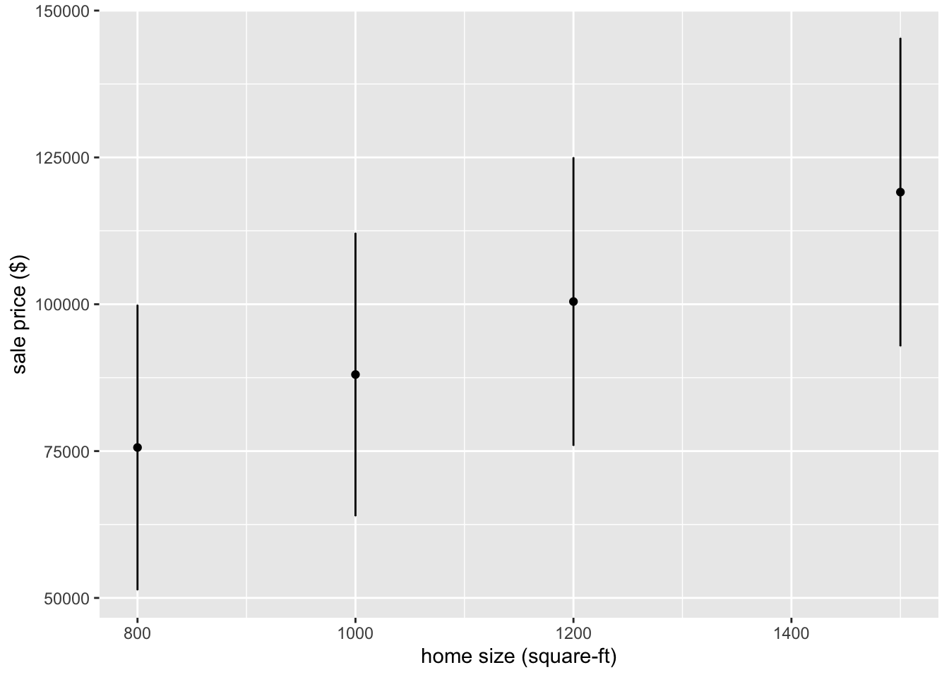
Fitting a Bayesian model
Re-purposing the previous fit() call is now straightforward. Notice that it is unchanged, we only need to define the new engine to operate on it.
First, set the prior distribution to be the default as discussed at Prior Distributions for rstanarm Models.
# set the prior distribution
prior_dist <-
  rstanarm::stan_glm(sell_price ~ beds + baths + home_size + year_built + lot_size,
                     data = smyrnaScrape, chains = 1) # using default prior means don't add
##
## SAMPLING FOR MODEL 'continuous' NOW (CHAIN 1).
## Chain 1:
## Chain 1: Gradient evaluation took 0.000125 seconds
## Chain 1: 1000 transitions using 10 leapfrog steps per transition would take 1.25 seconds.
## Chain 1: Adjust your expectations accordingly!
## Chain 1:
## Chain 1:
## Chain 1: Iteration: 1 / 2000 [ 0%] (Warmup)
## Chain 1: Iteration: 200 / 2000 [ 10%] (Warmup)
## Chain 1: Iteration: 400 / 2000 [ 20%] (Warmup)
## Chain 1: Iteration: 600 / 2000 [ 30%] (Warmup)
## Chain 1: Iteration: 800 / 2000 [ 40%] (Warmup)
## Chain 1: Iteration: 1000 / 2000 [ 50%] (Warmup)
## Chain 1: Iteration: 1001 / 2000 [ 50%] (Sampling)
## Chain 1: Iteration: 1200 / 2000 [ 60%] (Sampling)
## Chain 1: Iteration: 1400 / 2000 [ 70%] (Sampling)
## Chain 1: Iteration: 1600 / 2000 [ 80%] (Sampling)
## Chain 1: Iteration: 1800 / 2000 [ 90%] (Sampling)
## Chain 1: Iteration: 2000 / 2000 [100%] (Sampling)
## Chain 1:
## Chain 1: Elapsed Time: 1.3903 seconds (Warm-up)
## Chain 1: 0.110121 seconds (Sampling)
## Chain 1: 1.50042 seconds (Total)
## Chain 1:set.seed(123) # for reproducibiility
# make the parsnip model
bayes_mod <-
linear_reg() %>%
set_engine("stan",
prior_intercept = prior_dist$prior.info$prior_intercept,
prior = prior_dist$prior.info$prior)# train the model
bayes_fit <-
bayes_mod %>%
fit(sell_price ~ beds + baths + home_size + year_built + lot_size, data = smyrnaScrape)
print(bayes_fit, digits = 5)## parsnip model object
##
## Fit time: 1m 0.4s
## stan_glm
## family: gaussian [identity]
## formula: sell_price ~ beds + baths + home_size + year_built + lot_size
## observations: 493
## predictors: 6
## ------
## Median MAD_SD
## (Intercept) 215619.60310 6485.64949
## beds 0.08791 2.39662
## baths 0.01896 2.52481
## home_size 8.09597 2.51432
## year_built 0.09409 2.49585
## lot_size 0.01536 0.03170
##
## Auxiliary parameter(s):
## Median MAD_SD
## sigma 175173.11326 5667.42774
##
## ------
## * For help interpreting the printed output see ?print.stanreg
## * For info on the priors used see ?prior_summary.stanregtidy(bayes_fit, conf.int = TRUE)## # A tibble: 6 x 5
## term estimate std.error conf.low conf.high
## <chr> <dbl> <dbl> <dbl> <dbl>
## 1 (Intercept) 215620. 6486. 205193. 226538.
## 2 beds 0.0879 2.40 -4.11 4.12
## 3 baths 0.0190 2.52 -4.07 4.11
## 4 home_size 8.10 2.51 3.91 12.2
## 5 year_built 0.0941 2.50 -3.96 3.97
## 6 lot_size 0.0154 0.0317 -0.0350 0.0687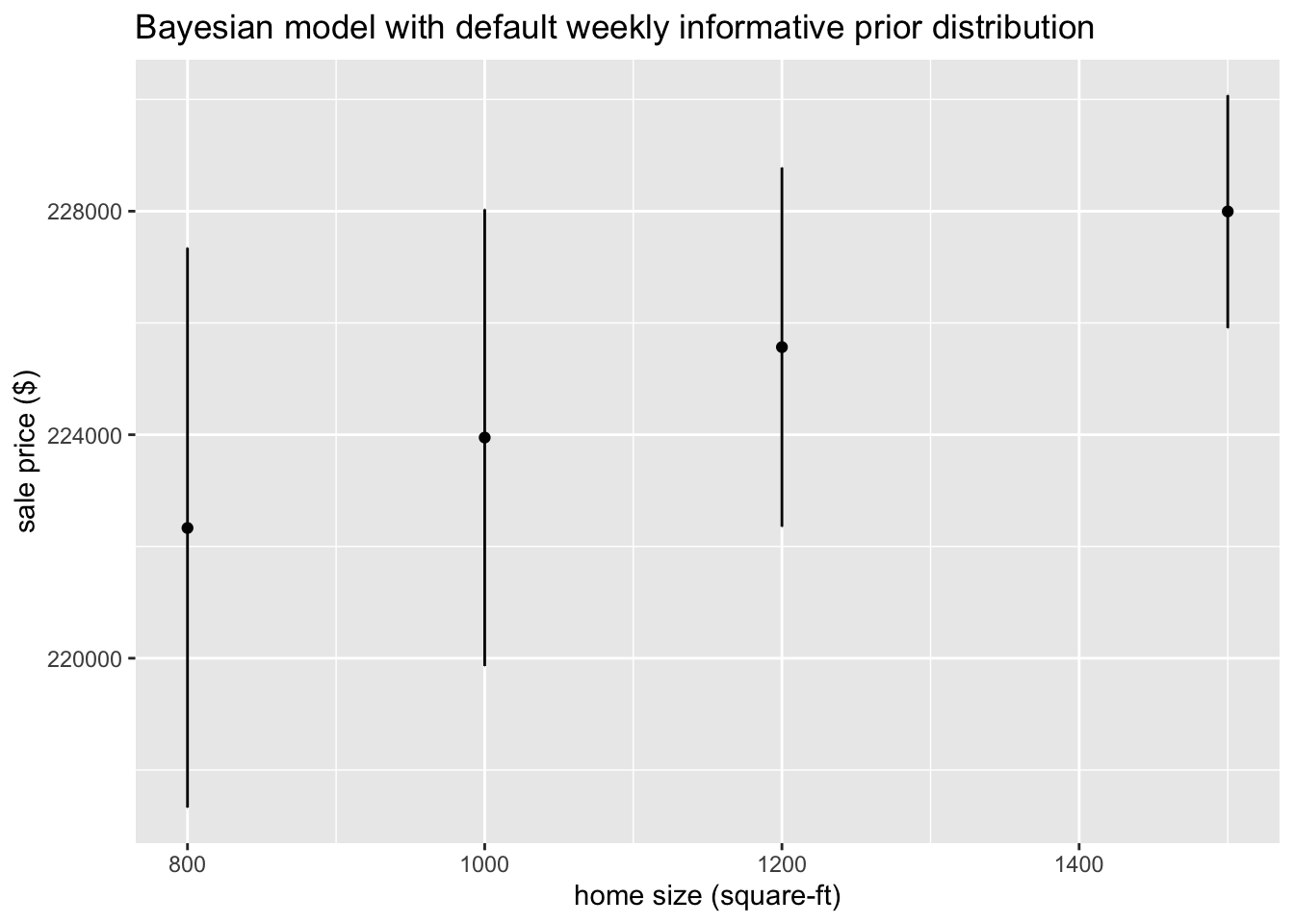 ## Using the
 tidymodels modeling workflow
Start by loading the data and filtering out really inexpensive and expensive recently sold homes that may skew predictions, then do some pre-processing before applying a machine learning method, including removal of data with missing values.
smyrnaScrape <-
  smyrnaScrape %>%
  # Remove heating/cooling vars until can figure out how to standardize
  select(-heating, -cooling, -parking) %>%
  # Filter out irrelevant "homes"
  filter(sell_price > 100000, sell_price < 750000) %>%
  # Exclude missing data
  na.omit()

# Convert home type to factor
smyrnaScrape$home_type <- factor(smyrnaScrape$home_type)
We can see how the average sell price varies by price.
## # A tibble: 5 x 3
##   group               n mean_sale
##   <fct>           <int>     <dbl>
## 1 [101000,150600)    92   130280.
## 2 [150600,186000)    89   168883.
## 3 [186000,220000)    81   203232.
## 4 [220000,284000)    87   248642
## 5 [284000,735000]    87   393459.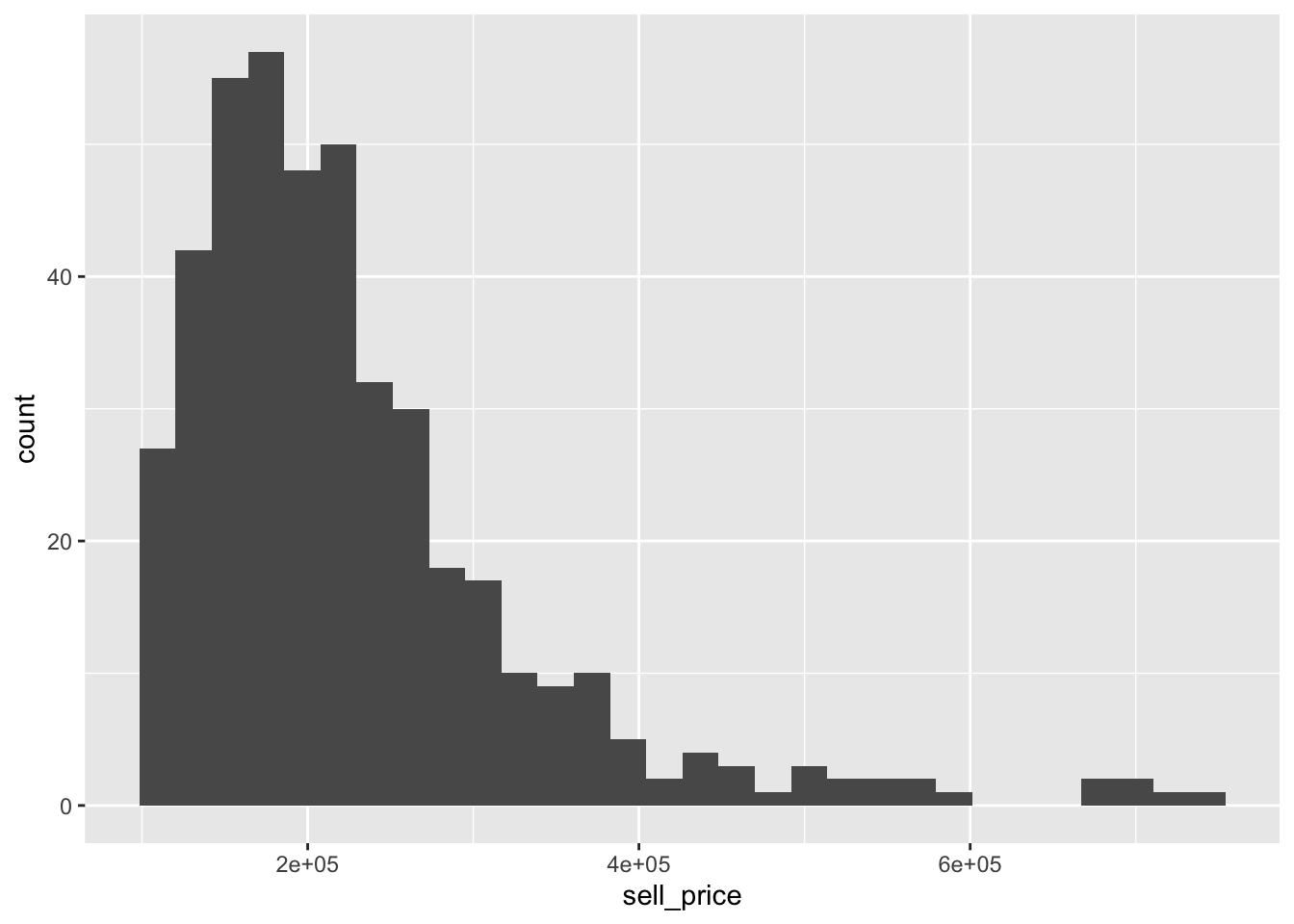
Data splitting
To get started, let’s split this single dataset into two: a training set and a testing set. We’ll keep most of the rows in the original dataset (subset chosen randomly) in the training set. The training data will be used to fit the model, and the testing set will be used to measure model performance.
To do this, we can use the rsample package to create an object that contains the information on how to split the data, and then two more rsample functions to create data frames for the training and testing sets:
# Fix the random numbers by setting the seed
# This enables the analysis to be reproducible when random numbers are used
set.seed(555)
# Put 3/4 of the data into the training set
data_split <- initial_split(smyrnaScrape, prop = 3/4)

# Create data frames for the two sets:
train_data <- training(data_split)
test_data  <- testing(data_split)
Create recipe and roles and finalize features
To get started, let’s create a recipe for a simple regression model. Before training the model, we can use a recipe to create a few new predictors and conduct some pre-processing required by the model.
Let’s initiate a new recipe and add a role to this recipe. We can use the update_role() function to let recipes know that address and home_type are variables with a custom role that we will call “ID” (a role can have any character value). Whereas our formula included all variables in the training set other than sell_price as predictors, this tells the recipe to keep address and home_type but not use them as either outcomes or predictors.
smyrna_rec <-
  # '.' means use all other vars as predictors
  recipe(sell_price ~ ., data = train_data) %>%
  update_role(address, home_type, new_role = "ID") %>%
  # Remove columns from the data when the training set data have a single value
  # I.e., if it is a "zero-variance predictor" that has no information within the column
  step_zv(all_predictors())
This step of adding roles to a recipe is optional; the purpose of using it here is that address and home_type can be retained in the data but not included in the model. This can be convenient when, after the model is fit, we want to investigate some poorly predicted value. ID columns will be available and can be used to try to understand what went wrong.
To get the current set of variables and roles, use the summary() function.
summary(smyrna_rec)## # A tibble: 8 x 4
## variable type role source
## <chr> <chr> <chr> <chr>
## 1 address nominal ID original
## 2 beds numeric predictor original
## 3 baths numeric predictor original
## 4 home_size numeric predictor original
## 5 home_type nominal ID original
## 6 year_built numeric predictor original
## 7 lot_size numeric predictor original
## 8 sell_price numeric outcome originalNow we’ve created a specification of what should be done with the data. How do we use the recipe we made?
Fit a model with a recipe
Let’s first use linear regression to model the flight data similar to what was done initially.
lr_mod <-
  linear_reg() %>%
  set_engine("lm")

smyrna_wflow <-
  workflow() %>%
  add_model(lr_mod) %>%
  add_recipe(smyrna_rec)

smyrna_wflow
## ══ Workflow ════════════════════════════════════════════════════════════════════
## Preprocessor: Recipe
## Model: linear_reg()
##
## ── Preprocessor ────────────────────────────────────────────────────────────────
## 1 Recipe Step
##
## ● step_zv()
##
## ── Model ───────────────────────────────────────────────────────────────────────
## Linear Regression Model Specification (regression)
##
## Computational engine: lmNow, there is a single function that can be used to prepare the recipe and train the model from the resulting predictors.
smyrna_fit <-
  smyrna_wflow %>%
  fit(data = train_data)
This object has the finalized recipe and fitted model objects inside. You may want to extract the model or recipe objects from the workflow. To do this, you can use the helper functions pull_workflow_fit() and pull_workflow_prepped_recipe(). For example, here we pull the fitted model object then use the broom::tidy() function to get a tidy tibble of model coefficients.
smyrna_fit %>%
  pull_workflow_fit() %>%
  tidy()
## # A tibble: 6 x 5
## term estimate std.error statistic p.value
## <chr> <dbl> <dbl> <dbl> <dbl>
## 1 (Intercept) -18064. 329766. -0.0548 9.56e- 1
## 2 beds 11580. 7271. 1.59 1.12e- 1
## 3 baths 35877. 9458. 3.79 1.78e- 4
## 4 home_size 42.3 6.51 6.49 3.23e-10
## 5 year_built 29.9 168. 0.178 8.59e- 1
## 6 lot_size 0.0170 0.0132 1.28 2.00e- 1Use a trained workflow to predict
Our goal was to predict the sale price of a home in New Smyrna Beach, FL. We have just:
Built the model (
lr_mod),Created a pre-processing recipe (
smyrna_rec),Bundled the model and recipe (
smyrna_wflow), andTrained our workflow using a single call to
fit().
The next step is to use the trained workflow (smyrna_fit) to predict with the unseen test data, which we will do with a single call to predict(). The predict() method applies the recipe to the new data, then passes them to the fitted model.
smyrna_pred <-
  predict(smyrna_fit, test_data) %>%
  bind_cols(test_data %>% select(sell_price, beds, baths, home_size))

smyrna_pred
## # A tibble: 109 x 5
## .pred sell_price beds baths home_size
## <dbl> <dbl> <dbl> <dbl> <dbl>
## 1 183573. 180000 2 2 1124
## 2 225640. 270000 3 2 1838
## 3 202140. 180000 3 2 1258
## 4 330313. 715000 4 4 2380
## 5 170477. 125000 2 2 810
## 6 190588. 218500 2 2 1290
## 7 198515. 227000 2 2 1468
## 8 139182. 169900 2 1 963
## 9 132655. 125900 2 1 804
## 10 299311. 535000 5 3 2245
## # … with 99 more rowsNow that we have a tibble with our predictions, how will we evaluate the performance of our workflow? We would like to calculate a metric that tells how well our model predicted late arrivals, compared to the true status of our outcome variable, sell_price.
smyrna_pred %>%
  rmse(sell_price, .pred)
## # A tibble: 1 x 3
## .metric .estimator .estimate
## <chr> <chr> <dbl>
## 1 rmse standard 105780.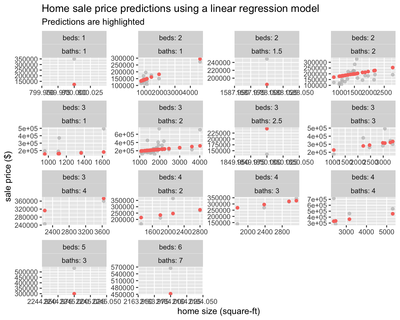
Moving to machine learning
Next, we will build on what we’ve learned and create a random forest model by simply defining a new workflow!
rf_mod <-
  rand_forest(trees = 1000) %>%
  set_engine("ranger") %>%
  set_mode("regression")

smyrna_rf_wflow <-
  workflow() %>%
  add_model(rf_mod) %>%
  add_recipe(smyrna_rec)
set.seed(234)
smyrna_rf_fit <-
smyrna_rf_wflow %>%
fit(data = train_data)
smyrna_rf_fit## ══ Workflow [trained] ══════════════════════════════════════════════════════════
## Preprocessor: Recipe
## Model: rand_forest()
##
## ── Preprocessor ────────────────────────────────────────────────────────────────
## 1 Recipe Step
##
## ● step_zv()
##
## ── Model ───────────────────────────────────────────────────────────────────────
## Ranger result
##
## Call:
## ranger::ranger(formula = ..y ~ ., data = data, num.trees = ~1000, num.threads = 1, verbose = FALSE, seed = sample.int(10^5, 1))
##
## Type: Regression
## Number of trees: 1000
## Sample size: 327
## Number of independent variables: 5
## Mtry: 2
## Target node size: 5
## Variable importance mode: none
## Splitrule: variance
## OOB prediction error (MSE): 4817952011
## R squared (OOB): 0.472358smyrna_rf_pred <-
predict(smyrna_rf_fit, test_data) %>%
bind_cols(test_data %>% select(sell_price, beds, baths, home_size))
smyrna_rf_pred## # A tibble: 109 x 5
## .pred sell_price beds baths home_size
## <dbl> <dbl> <dbl> <dbl> <dbl>
## 1 152816. 180000 2 2 1124
## 2 214435. 270000 3 2 1838
## 3 209350. 180000 3 2 1258
## 4 348550. 715000 4 4 2380
## 5 145537. 125000 2 2 810
## 6 189050. 218500 2 2 1290
## 7 185739. 227000 2 2 1468
## 8 180856. 169900 2 1 963
## 9 181623. 125900 2 1 804
## 10 348442. 535000 5 3 2245
## # … with 99 more rows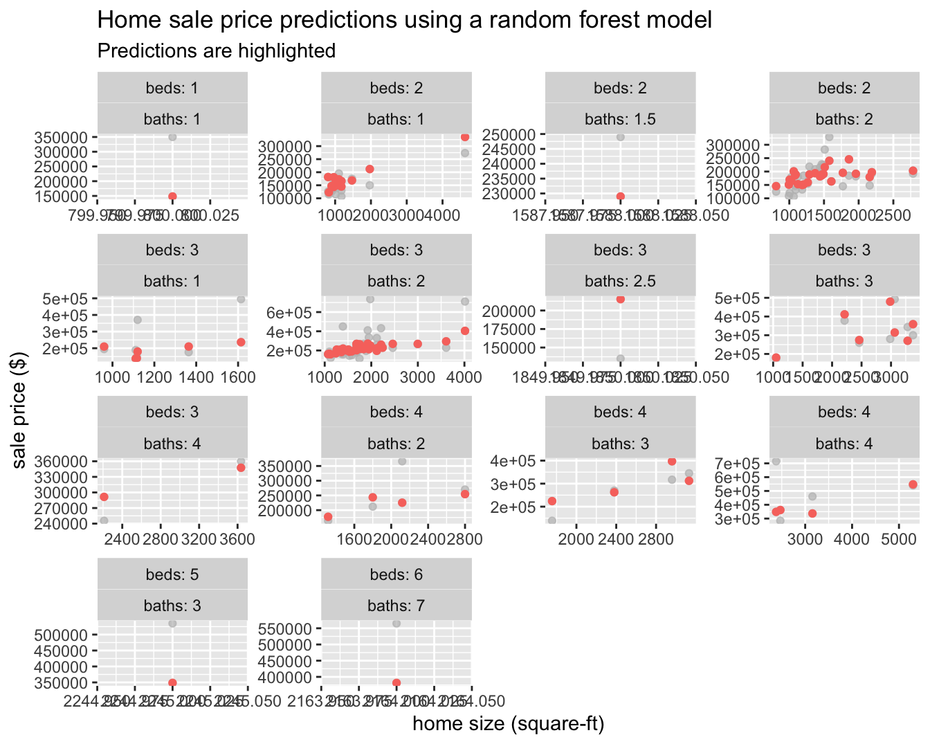
We can now see that some of the structure in the data is being picked up compared to the linear regression model, which can only represent a line of best fit through the data.
Let’s try and predict the sale price of 1160 Fairvilla Dr, New Smyrna Beach, FL 32168 using both models.
new_data = data.frame(address = c("1160 Fairvilla Dr, New Smyrna Beach, FL 32168"),
                      beds = c(2),
                      baths = c(1),
                      home_size = c(816),
                      home_type = c("Single Family"),
                      year_built = c(1985),
                      lot_size = c(816))

bind_cols(predict(smyrna_fit, new_data) %>% rename(lm = .pred),
          predict(smyrna_rf_fit, new_data)%>% rename(rf = .pred)
)
## # A tibble: 1 x 2
## lm rf
## <dbl> <dbl>
## 1 134824. 126690.The Zestimate for this property (as of this writing) is $115,170 with a range of $105,000 - $124,000 with a list price of $125,000. Both of our models fit are outside of the Zestimate range, but the sale price estimate from the random forest model is just outside of it. This is really not surprising as we did not go out of our way to add any sophistication to our feature set and we are only working with 436 data points, but it is still good to be close with such little effort!
Of course the real validation point will be the actual sale price 😉.